Support Vector Machines (SVM): Intuition and Classification Explained

An introduction to Support Vector Machines (SVM), exploring concepts such as VC dimension, hyperplanes, support vectors, soft margins, the kernel trick, and multiclass classification.

Support Vector Machines (SVM) are versatile algorithms widely used for classification and regression problems. In this post, the focus will be on developing an intuitive understanding of how SVM works in classification tasks.

The goal here is to present the main concepts behind the algorithm in an accessible way, avoiding overly formal mathematical demonstrations. Rather than covering every theoretical detail, the objective is to build a solid intuition for the logic behind SVM, from the idea of separation through hyperplanes to the use of the kernel trick.

By the end of this post, you will have a clear understanding of the algorithm’s purpose, its main characteristics, and the contexts in which it is commonly applied.

Vapnik-Chervonenkis (VC) Dimension

The Vapnik-Chervonenkis (VC) dimension is a measure used to quantify the representational capacity of a classification model. Intuitively, it indicates the maximum number of points that can be correctly separated in every possible configuration (shattering) by a given set of functions.

This concept was introduced by Vapnik and Chervonenkis in 1971 and is widely used to analyze the flexibility of statistical learning models. In general, the higher the VC dimension, the greater the model’s ability to represent complex patterns.

Example

The VC dimension of binary linear classifiers in a two-dimensional plane is equal to 3. This means that there are configurations of 3 points that can be correctly separated in all possible label combinations using a straight line.

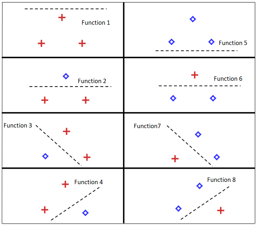
Illustration of Vapnik-Chervonenkis (VC) dimension in SVM classification

However, when using 4 points, there are already some configurations that cannot be separated by a single linear function.

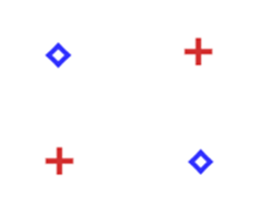
Illustration of binary classification using four separable points

This measure is important because models with a very high VC dimension tend to memorize the data (overfitting), while models with a VC dimension that is too low may fail to learn relevant patterns (underfitting).

Hyperplane

A hyperplane divides the feature space into decision regions associated with different classes.

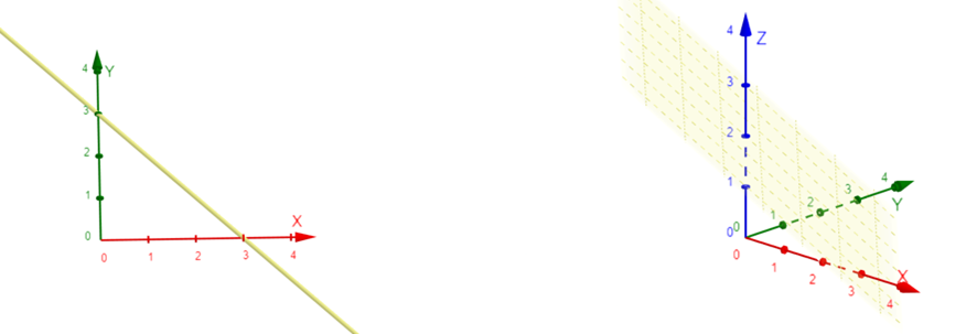
A hyperplane is a geometric structure of dimension $ (k - 1) $ embedded in a space of dimension $ (k) $. Intuitively:

in a two-dimensional space, a hyperplane corresponds to a line;
in a three-dimensional space, it corresponds to a plane;
in higher dimensions, it is the generalization of these ideas.

Illustration showing that a hyperplane is a line in two dimensions and a plane in three dimensions

Connecting this idea with the previous topic, linear classifiers defined by hyperplanes in a space of dimension $ (K) $ have a VC dimension equal to $ (K + 1) $ . This helps explain the capacity of these models to separate different data configurations.

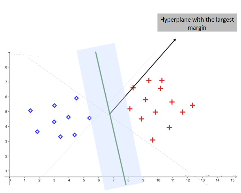
In many classification problems, there are multiple hyperplanes capable of correctly separating the classes:

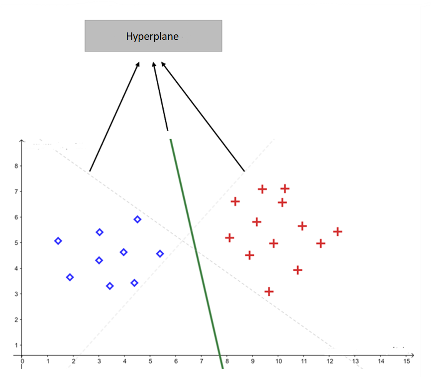
Example of a separating hyperplane in Support Vector Machines

The goal of SVM is to find the hyperplane that maximizes the separation margin between the classes. In other words, the algorithm searches for the decision boundary that is as far as possible from the points of both categories.

A large margin acts as a “safety buffer”: the larger the margin, the more robust the classifier tends to be against noise and unseen examples.

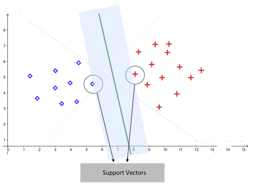
Support Vector Machine hyperplane with maximum margin between classes

Support Vectors

Support vectors are the data points closest to the separating hyperplane. They are the points that define the classifier’s maximum margin and, consequently, directly influence the position of the optimal hyperplane found by SVM.

These points are called “support vectors” because they support the model’s decision boundary. In practical terms, small changes in these points can significantly alter the resulting hyperplane.

An important characteristic of SVM is that only the support vectors directly participate in defining the final solution. Points located farther from the decision boundary have little or no influence on the optimal hyperplane.

Support Vectors

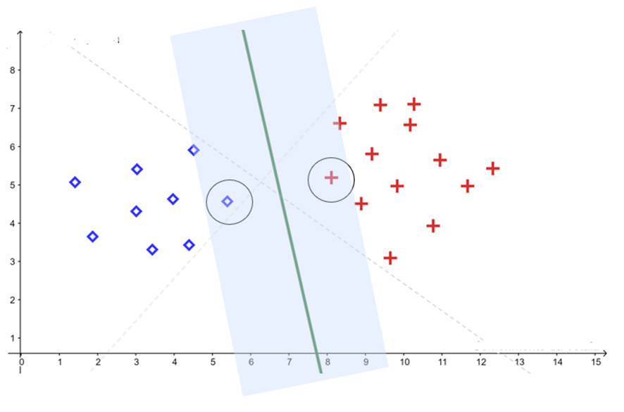
Soft Margins

In many real-world problems, the data cannot be perfectly separated by a hyperplane. To handle this scenario, SVM can use soft margins, allowing some points to invade the separation margin or even be misclassified.

This flexibility reduces the rigidity of the model and helps prevent overfitting, making the classifier more robust to noise and outliers.

SVM therefore seeks a balance between:

maximizing the separation margin;
minimizing classification errors.

Illustration of soft margins in Support Vector Machines

This balance is controlled by the hyperparameter $ (C) $:

High $ (C) $ → strongly penalizes errors → rigid margin → higher risk of overfitting
Low $ (C) $ → tolerates violations → softer margin → better generalization

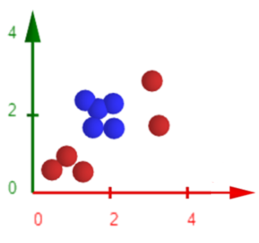
But what happens when the data cannot be separated linearly?

Nonlinear Data and Cover’s Theorem

Cover’s Theorem states that complex patterns are more likely to become linearly separable when projected into higher-dimensional spaces, provided that these spaces are not excessively populated.

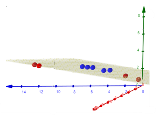
Illustration of nonlinear data and feature space transformation in Support Vector Machines

Based on this idea, we can apply transformations to the data in order to map it into a new feature space with higher dimensionality. For example, a transformation such as:

\[(x, y) \rightarrow (x^2, \sqrt{2}xy, y^2)\]

can make separable a dataset that was originally not linearly separable.

After this transformation, it becomes possible to apply a linear SVM in the new feature space.

Illustration of feature space transformation in Support Vector Machines

However, explicitly working in high-dimensional spaces can be computationally expensive. This challenge motivated the development of the so-called kernel trick, which allows these transformations to be performed implicitly and efficiently.

Example: Quadratic Polynomial Kernel

Consider the following kernel:

\[K(\mathbf{w}, \mathbf{q}) = (\mathbf{w}^T \mathbf{q})^2\]

Expanding the inner product:

\[= (x_1x_2 + y_1y_2)^2\] \[= x_1^2x_2^2 + 2x_1x_2y_1y_2 + y_1^2y_2^2\]

This expression can be rewritten as:

\[= \phi(\mathbf{w})^T \phi(\mathbf{q})\]

where:

\[\phi(x,y) = (x^2,\sqrt{2}xy,y^2)\]

In other words, the kernel implicitly computes the inner product in a higher-dimensional space, without the need to explicitly calculate the transformation $ (\phi) $.

This makes training computationally more efficient, especially when working with very large feature spaces.

Types of Kernels

There are several types of kernel functions commonly used in SVM, among the most well-known are:

Linear Kernel;
Polynomial Kernel;
Radial Kernel (RBF);
Sigmoid Kernel (Hyperbolic Tangent).

Each kernel implicitly defines a different type of transformation of the feature space.

Polynomial Kernel

The polynomial kernel allows the representation of nonlinear decision boundaries through polynomial combinations of the features.

\[K(\mathbf{x}, \mathbf{y}) = (\gamma \mathbf{x}^T \mathbf{y} + c)^d\]

where:

$ (d) $ defines the degree of the polynomial;
$ (\gamma) $ controls the influence of the data;
$ (c) $ is an adjustment constant.

Radial Kernel (RBF)

The radial kernel (Radial Basis Function) is one of the most widely used kernels in SVM because of its ability to model highly nonlinear relationships.

\[K(\mathbf{x}, \mathbf{y}) = e^{-\gamma \|\mathbf{x}-\mathbf{y}\|^2}\]

This kernel measures similarity based on the Euclidean distance between points: the closer the points are, the higher the kernel value tends to be.

Sigmoid Kernel (Hyperbolic Tangent)

The sigmoid kernel behaves similarly to artificial neurons used in neural networks.

\[K(\mathbf{x}, \mathbf{y}) = \tanh(\gamma \mathbf{x}^T \mathbf{y} + c)\]

Its use is less common compared to polynomial and radial kernels.

But what happens when we have more than two classes?

Multiclass SVM Classification

SVM was originally developed for binary classification problems. However, several strategies allow its extension to scenarios involving multiple classes.

SVM Multiclasse

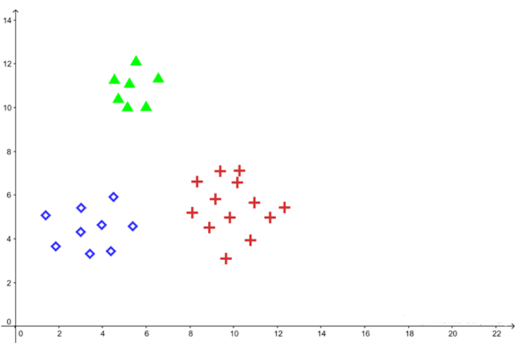
Among the main methods used, the following stand out:

One-vs-Rest (OvR)

In this method, a classifier is trained to separate one specific class from all the others. The process is repeated for each class in the problem.

For example, in a problem with three classes $ (A) $ , $ (B) $ , and $ (C) $ , three classifiers would be trained:

$ (A) $ versus $ ((B, C)) $ ;
$ (B) $ versus $ ((A, C)) $ ;
$ (C) $ versus $ ((A, B)) $ .

One-vs-One (OvO)

In this approach, a classifier is trained for every possible pair of classes.

In a problem with three classes, classifiers would be trained for:

$ (A) $ versus $ (B) $ ;
$ (A) $ versus $ (C) $ ;
$ (B) $ versus $ (C) $ .

The final decision is usually made through a voting process among the classifiers.

DAG-SVM

DAG-SVM (Directed Acyclic Graph SVM) organizes multiple binary classifiers into a directed acyclic graph structure based on sequential binary classifications.

At each stage, one class is eliminated until only the final class assigned to the example remains.

References:

Shalev-Shwartz, Shai, and Shai Ben-David. Understanding Machine Learning: From Theory to Algorithms. Cambridge University Press, 2014. [link]
Faceli, Katti. Inteligência artificial: uma abordagem de aprendizado de máquina. Grupo Gen - LTC, 2011.
Cover, Thomas M. “Geometrical and Statistical Properties of Systems of Linear Inequalities with Applications in Pattern Recognition.” IEEE Transactions on Electronic Computers, vol. EC-14, no. 3, June 1965, pp. 326–34. DOI.org (Crossref), https://doi.org/10.1109/PGEC.1965.264137. [link]
Chih-Wei Hsu and Chih-Jen Lin. “A Comparison of Methods for Multiclass Support Vector Machines.” IEEE Transactions on Neural Networks, vol. 13, no. 2, Mar. 2002, pp. 415–25. DOI.org (Crossref), https://doi.org/10.1109/72.991427.
Platt, John and Cristianini, Nello and Shawe-Taylor, John. “Large Margin DAGs for Multiclass Classification”. Advances in Neural Information Processing Systems, MIT Press, vol.12, 1999. [link]
V.N. Vapnik and A.Ya. Chervonenkis. Theory of Pattern Recognition. Nauka, Moscow, 1974. (in Russian); German translation: Theorie der Zeichenerkennung, Akademie Verlag, Berlin, 1979.